Geometry effects; hedging your bet on emissivity!

InfraMation 2003 Application Paper Submission

Mikael Cronholm

ABSTRACT  

In this paper I will describe a way to improve measurements on low emissivity targets where it is  necessary to guess emissivity. As all thermographers who have been through ITC’s training courses  know, emissivity is influenced by six factors – material, surface structure, viewing angle, geometry,  wavelength, and temperature. Most of us would probably agree that material and surface structure are  the most important of those. After some recent experience and some simple research, I have personally  started to appreciate the geometry factor more. In fact, I feel an urge to discuss this with the IR  community, because it seems to me that in some situations, geometry could be our saving grace out  there. Our job is often a bit of a gamble, especially in those cases when emissivity of the material itself is  low, for example in indoor HV substations.  

We all know the principle of a blackbody cavity, and it is when the shape of the target starts to resemble  such a cavity that geometry gives us an advantage.  

One of the difficulties with using the geometry factor is that it is quite difficult to know exactly how much  emissivity will increase as the shape of the target approaches that of a blackbody cavity. Then it is time  for some clever deductive reasoning on our part! It is time for using the camera for playing a bit of “What  if?” – something that I am personally very fond of, since I find that it helps me improve my work a great  deal.  

THE PROBLEM  

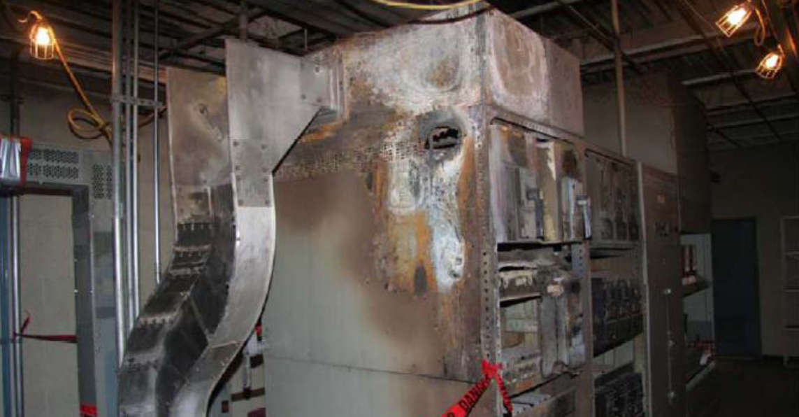
In our daily lives as thermographers, we frequently have to guess emissivity, especially if we work on  electrical equipment under load, because we cannot touch the components. One of the more difficult  cases involves high voltage equipment indoors. We have low emissivities because the environment is  usually quite clean, and it is common that the equipment is bare metal. Additionally, the size of the  conductor is often quite large compared to the current flow, which means the components don’t heat up  much due to the load. The consequence is that it may be difficult just to find a thermal anomaly, and once  it is found, it will be difficult to measure its temperature with some degree of accuracy.  

How damaging is a wrong guess of emissivity?  

During my training courses we often do an exercise where I pass around pieces of metal, like copper bus  bars with varying degrees of oxidation, and then let the students guess the emissivity. That is usually a  humbling and shocking experience that illustrates the difficulties very well. If you have not done it, pick up  some pieces and try! Be honest to yourself when you guess, and then do a measurement of the  emissivities. The next thing you may want to do is to input your guess, and see how wrong your  measurements would have been if you had used your guess. You will notice that at very low emissivities,  a small emissivity error will cause a large measurement error. At higher emissivity it is more forgiving.  

Let’s look at the following examples to get this into perspective. The tables below were made using a  FLIR ThermaCAM P60 instrument. Different camera models will give different results if you recreate this  experiment, and because cameras are individually calibrated, even another ThermaCAM P60 may give  slightly different results. The principle will always be the same though. 

In this example I have assumed a true target temperature of 80°C. That is not a completely arbitrary  choice. In many situations, that is a critical threshold level for classifying an anomaly. Above 80°C may be  a critical problem, whereas a lower temperature is deemed less critical. I have also assumed correct  emissivities of 0.10 to 0.90, in 0.10 step increments. The other parameters were set as follows: Reflected  apparent temperature at 20°C, air temperature at 20°C, distance at 3 meters, and relative humidity at  50%. For each assumed correct emissivity, I have varied the emissivity in 0.10 increments and recorded  the resulting temperature reading, to simulate different wrong guesses of emissivity.  

The bolded values are the ones where the correct (assumed) emissivities are entered. TM is the  measured temperature at that emissivity setting, and ∆T stands for the measurement error. For example,  if the true emissivity is 0.70, and we erroneously input an emissivity of 0.50, we will be reading a  temperature of 98.2°C, and our error will be +18.2 K. 

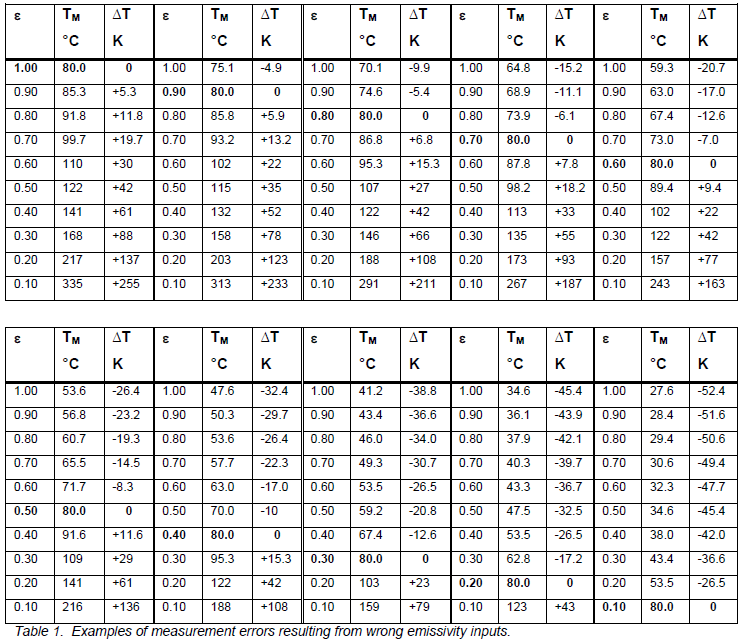
The errors at lower emissivities don’t look very large numerically speaking, but when you look at the  increase in temperature over that of the surroundings (20°C), the errors seem relatively more significant.  For example, our 80°C temperature at an emissivity of 0.10 melts down to just 28.4°C at an emissivity of  0.90. What is an acceptable error depends on your application and what your target is. But if your true  emissivity goes below about 0.60 or 0.50, there is not much room for error anymore, if you want to stay  within ± -10 K from the actual temperature.  

WHAT INFLUENCES THE EMISSIVITY OF THE TARGET?  

Here is the list of factors that have an influence:

1. Material  

2. Surface structure  

3. Geometry of the target  

4. Viewing angle  

5. Wavelength of the camera  

6. Target temperature

The list is in a rough order of importance, but it will vary from one situation to another. What we prefer is  an emissivity that is as high as possible – if everything had an emissivity of 1.0, our job would be a lot  easier! But that is not the way it is.  

Let’s consider a situation where the material is a metal, not much corroded, and fairly smooth on the  surface. In such a situation, the first two factors will not supply us with much, as far as emissivity is  concerned. If we skip over geometry for now, and consider the other three – angle, wavelength, and  temperature – how much help can we get from them? As we shall find out, not much!  

If we look at viewing angle first, it may raise the emissivity slightly if we pick an ideal angle compared to a  bad one. But angle will never make a very big difference. If it does, it usually lowers the emissivity even  further, as we move towards an oblique angle. The angle dependency is also connected to the surface  structure, and with a smooth surface it will be less likely that viewing angle will help us. This is a subject  for an entire paper in itself, so I will leave it at that for now.  

A metal surface is unlikely to have an emissivity that changes much with wavelength.¹ Theoretically, you  will get slightly higher emissivity with a shortwave camera than a longwave. But as a general rule, a  clean, smooth metal surface will have a very low emissivity in both wavelengths, varying between 0.02  and 0.20. The important thing to remember about the wavelength factor is that an emissivity  measurement made with one camera may not be valid for a measurement with another. Most of us have  one camera, and that’s it. 

The temperature of the target may change the emissivity a few points, but you will most likely have to  change the temperature several hundred Kelvin to make a difference.1 And besides, the temperature of  your target is what it is, and that is what you need to measure. So the relevance of this factor is a bit  similar to wavelength; you need to measure your emissivity at roughly the temperature where you will be  measuring temperature later, and if that is a low emissivity…well, you are stuck with it!  

The geometry factor  

Let’s turn to what I like to call our saving grace, the geometry factor. I have come to appreciate this factor  more and more, and I would go as far as saying that without it, many of our targets would hardly have  much of an emissivity at all.  

To understand how this factor works, we may want to have a look at the way a blackbody reference  source works. The technical solution that is sometimes used is based on the geometry factor to give it  that very last bit of emissivity that material and surface structure alone cannot supply.

Let us first remind ourselves of Kirchhoff’s Law of unity, which states that, the emissivity of a surface or  body will be directly proportional to the absorptivity of that surface or body. In other words, a good  absorber will also be a good emitter.  

The figure below is a cross section of a so-called inverted conical cavity. It is designed in such a way that  it will trap radiation that all, the surface material and structure are chosen to be favorable, so that the  emissivity would be high, even if it were a flat surface. Let’s say it would an emissivity/absorptivity of 0.98  if it were flat. That means that, provided of course that it is opaque, it will have a reflectivity of 0.02. 

Ninety-eight percent of the radiation that enters the inverted conical cavity will be absorbed and only 2%  reflected. The reflected radiation will not be reflected away from the cavity, as it would from a flat surface,  but towards another part of the interior of the cavity. At that point, 98% of the 2% will be absorbed, which  means that 0.04% of the radiation is left unabsorbed. After another reflection, 0.0008% will be left, and  that’s not very much. The angles of the cavity are chosen smartly, so that any angle the radiation enters,  it will be reflected back and forth inside the cavity, until it is virtually completely absorbed.  

Consequently, if we take the device and heat it up to a certain temperature, it will radiate with an intensity  that is almost exactly the same as a blackbody would at that very same temperature. We have created a  very good blackbody cavity. 

But between those two extremes – the flat surface and the inverted conical cavity – there are plenty of  variations of the theme. There are a lot of shapes that will give certain contributions to the total emissivity  of the target; angles, holes, slits, cracks, parallel surfaces, etc. If the material and surface conditions are  favorable, the geometry factor matters less, but if they are not, we can be greatly helped by geometry.  

So, where do I find different geometries in my emissivity tables? Well, emissivity tables aren’t that great to  start with, and you will not likely find anything that will tell you much about geometry in them. They usually  deal with flat surfaces. Doesn’t that make it pretty useless – if I don’t know the emissivity of a geometrical  shape, I still cannot measure the temperature! What should I do?  

EFFECTS OF GEOMETRICAL SHAPE OF A TARGET – EXAMPLES  

To illustrate the effects of geometry, I dug up some scrap pieces of metal, and I went to the hardware  store and bought some brand new nuts and bolts, pretended my kitchen was a lab for other things than  protein, and I did some experimenting. I used my oven to heat up the pieces as evenly as I could; with  electrical tape (Scotch Super 33+, using ε = 0.95) on strategic spots to enable temperature measurement  of the various geometrical shapes I had on my pieces. Here is what I concluded.  

(General notes: I use an emissivity setting of 1.00 for the images, and individual settings for each  measurement function I insert. Very often, the closest emissivity setting did not give me an exactly equal  temperature to that of the tape. In those cases I picked the emissivity that gave me the closest  temperature. That temperature is the one displayed in the IR image for the measurement function in  question.)  

First example: Bolted bus bar connection with low emissivity on flat surfaces  

The part is made of copper. On one side of it I kept the natural patina of the piece. It is not extremely  oxidized, but rather what you may expect after a few years of indoor service in normal conditions – not  very clean, not very dirty or corrosive surroundings. On the other side, I used some fine grain sandpaper  to remove the oxide. At the same time, I believe the surface may have become slightly rougher, but not  much. It is worth noting that the edges are rounded, not flat. I made a bolted T-joint, using brand new,  zinc plated bolt, nut, and washers.  

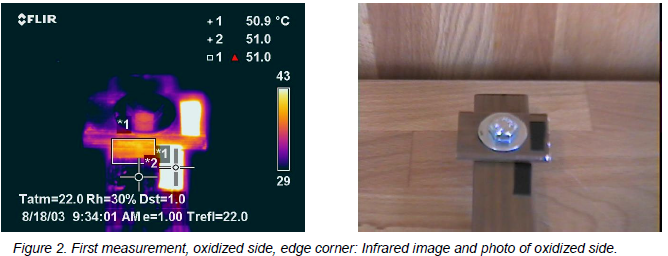
Spot 1 is on the tape and reads 50.9°C. Spot 2, on the flat copper, gave me an emissivity reading of 0.17,  and AreaBox 1, in the “geometry-corner” between the bus bar pieces, gave an emissivity of 0.60. I  consider that a very big difference! Looking back at the tables above, we can easily conclude that we will  be on much thinner ice trying to measure temperature around 0.17, than at 0.60. Playing “what if” with the  camera I get the following result: Guessing ± -0.10 wrong on emissivity at 0.60 will give us a reading of  47.3 to 56.1°C, a span of 8.8 K with 51.0°C being the correct value. Not too bad at all. Making the same  mistake at emissivity 0.17 will have the following result. At emissivity 0.27 I read 41.1°C, and at 0.07 I get  83.6°C. That is a span of 42.5 K with 51.0°C being the correct value. Not quite as good. I have to be able  to guess within roughly 0.14 to 0.20 (i.e ± -0.03) in emissivity to get the same accuracy as I would get with  a span of ± -0.10 around emissivity 0.60. I know I can guess that well on this particular piece, but only  because I make about thirty measurements per year on it during classes. I would be less confident in the  field!  

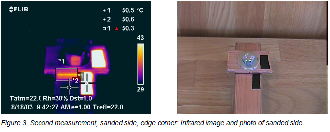
I was surprised myself by the results here! The emissivity increased more from the greater roughness,  than was lost with the removal of the oxide layer. The flat copper surface was 0.21. Interestingly, the  corner was still about 0.60, reading a temperature of 50.7°C, and in fact slightly higher than that. An  emissivity of 0.61 (which is set in the image above) gives a temperature of 50.3°C. Playing “what if” will  give similar results as previously.

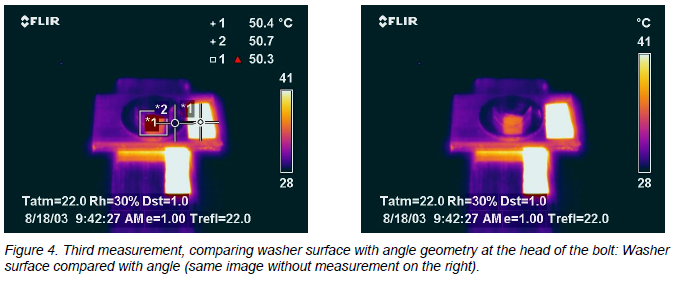
The flat washer, reflecting only the surrounding apparent temperature, has an emissivity of 0.19. In the  corner of the bolt and the washer (the area box), the emissivity is 0.46. I consider that to be a fairly decent  increase, just from the shape of the target. Again, it puts us in a less sensitive measurement situation,  with less potential for error due to wrong emissivity guessing. When you make a bet, try to get the best  odds you can!  

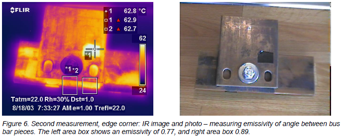
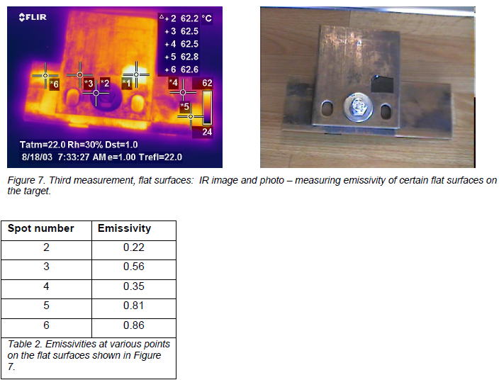
Second example: Bolted bus bar connection with comparatively higher emissivity on flat surfaces  

The copper pieces I used for this example are slightly more weathered. The discoloration is greater and it  is also unevenly distributed over the surfaces. The area on the bottom piece that extends below the top  piece with the two visible holes in it, and right at the angle where they meet, is roughed up with a grinder  of some sort before it was “aged”. So in all fairness, the holes and angles are not comparable to the flat  surface in this case, as they were in the previous. So don’t compare too much with the flat surfaces! Just  view this as an example of some emissivities created by a combination of material, surface condition, and  geometry. Emissivities of the flat surfaces are only supplied to satisfy your curiosity in general.  

The complete assembly is assumed to have a uniform temperature of 62.8°C, measured at the tape (spot meter 1).  

The holes are punched through the top piece, but stop at the one below, creating a cavity. The bottom  piece has a rougher surface at the right hole, which is why the resulting emissivity is higher there. 

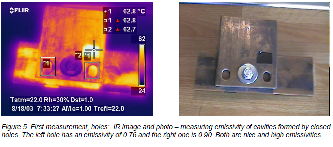
The target has many different emissivities, and some are high in themselves, without having any  geometrical shape that increases emissivity. But the two highest emissivities are from “geometrically  enhanced” shapes, and the lowest emissivities are at flat surfaces.  

Third example: Holes in cable shoes  

Many cable shoes have little peep holes to let you see the end of the cable before it is crimped, to make  sure it is inserted properly. Those holes make nice little blackbody cavities, provided you look at the right  angle. I have found them to be very useful in the field.

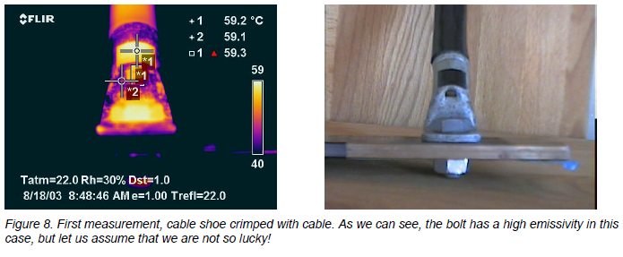
The tape gives us a temperature of 59.2°C, and using this temperature, I get an emissivity of 0.89 in the  hole, and 0.63 on the surface of the cable shoe, next to the hole.

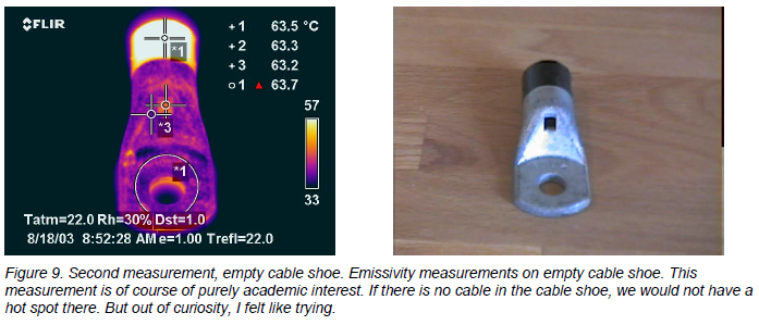
The temperature at the tape is 63.5°C. The surface next to the hole has an emissivity of 0.33. This  increases to 0.56 in the hole. That is less than the previous example, which is expected, because the  other end of the cable shoe is open to the surroundings. As an additional illustration of geometry effects,  the inner edge of the hole (area circle) has an emissivity of 0.61. 

CAN THE EFFECT OF GEOMETRICAL SHAPE BE PREDICTED?  

To illustrate this issue, I made some tests with a piece of aluminum that I normally use in class to illustrate  the existence of geometrical effects. It has a number of holes drilled in it. They are 10 mm wide and have  varying depths. Other than that, they should be similar as far as surface structure goes.

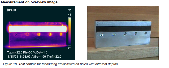
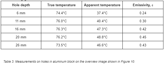
The true temperature varies a bit. It goes down towards the edges, which is natural, since it looses more  heat there. It also seems natural that the area around the 26 mm hole is cooler than around the 6 mm  hole, since the deeper hole looses more heat. The emissivity goes up as the holes get deeper, from 6 mm  to 20 mm, but then it goes down slightly. As we shall see, this is due to viewing angle.  

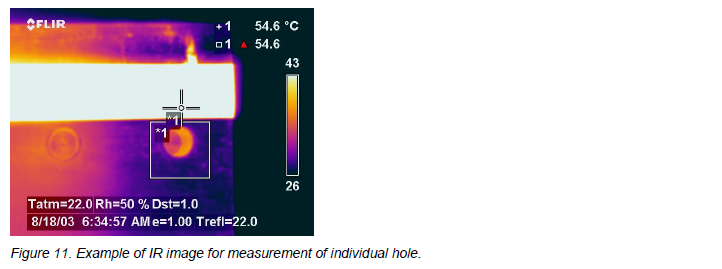
Individual measurements on the holes  

On each hole, I did a number of measurements, moving the camera around to try and pick off the highest  apparent temperature. I did not allow myself to use a perpendicular angle, because then I would reflect  myself and the camera, and the Treflected I used would be invalid. Figure 11 is an example of one of the  images. As you can see to the left, I am just avoiding reflecting myself in the target. 

The table below shows the emissivities I obtained, together with the ones from the overview image.  

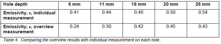
The result from this exercise was an increase in emissivity in all cases, and the greatest increase was on  the shallowest hole. I also got the expected rise in emissivity with hole depth, since I was using a more  ideal angle. The chart below shows individual emissivity measurements, plotted with the depths. I also  input a rough average of the emissivity of the flat surface (0.16).  

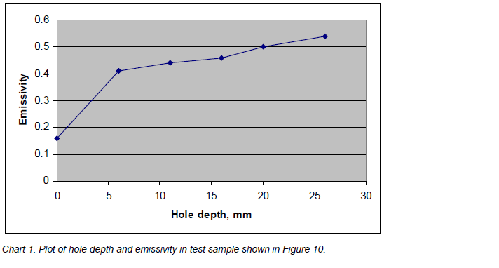
The shallowest hole is 6 mm deep, but it should be noted that the bottom of the hole is conical, from the  drill bit, so the sides of the hole are barely half that deep. What I am trying to say is that this hole doesn’t  look like much of a cavity at all, but still gives a good increase in emissivity.  

Going back to the original question; can we predict the emissivity of a geometrical shape? No, I  personally don’t believe we can. Theoretically, perhaps we could, but not in a way that will give us a  precise emissivity setting that we can use in the field. But on the other hand, how easy is it to guess  emissivity of a flat surface? A geometrical shape will always, I repeat ALWAYS, have an emissivity that is  higher than it would have if it were a flat surface. At the end, it will all come down to your experience.  

GEOMETRY AND SURFACE STRUCTURE  

Geometry and surface structure are very much related. What we call “surface structure” is in fact  thousands of little geometries repeated over a flat surface. For example, if we take a polished piece of  metal and sand blast it, every little recess that the grains of sand make will create a small cavity that  increases emissivity locally in that point. When we view it with our camera, all those little cavities blend  together into a single, higher emissivity. That’s surface structure. If, on the other hand, we bend the piece  of metal in an angle, we have created a different geometry, still maintaining the same surface structure.  

Surface structure, therefore, should not be mixed up with for example the degree of corrosion. When  something corrodes, it is the material factor that changes. However, corrosion has a tendency of  changing the surface structure as well, because the surface gets pitted, develops scaling, etc. But it is  important to remember what is what. Corrosion is the cause, but it has to separate consequences that are  two different things.

IF IT CAN’T BE PREDICTED, WHAT’S THE USE?  

First of all, anything that increases emissivity is welcome. A lot of times, we look at shiny components and  wonder if there is anything that is hot at all. Finding the hot spot is even more important than measuring  its temperature. When we analyze the image, we look at apparent temperature only, and if the emissivity  is very low, we may not actually see a difference in temperature between two connections, even if they  are in fact different. Instead of looking at shiny bus bars, we can concentrate on similar geometrical  shapes, and just compare the thermal signal, to determine if there is an anomaly there or not.  

Improving your odds by playing some more “what if”  

If you think two places on a target have a similar temperature, using your knowledge of heat transfer, the  point that emits the most radiation will have the highest emissivity. It doesn’t matter why! That is the place  where it will be easier to obtain a good measurement result. That is also the place where you can  determine the “rock-bottom temperature” for the target. This is how you can do it.  

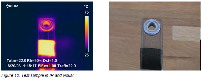
Let’s use this piece of copper bus bar shown in Figure 12 as an example. It has a threaded stud riveted to  it, and with some knowledge of how geometry works, we can conclude that it will have some interesting  shapes that will be favorable for emissivity. It also has a piece of tape on it, to enable our emissivity  measurement for this test. 

I heat it up and get the thermogram. I use this image and the tape to obtain the emissivity of the flat  surface between the tape and the riveted stud. The emissivity is 0.10. Let’s say I want to measure on the  flat surface, and I am guessing that the emissivity is 0.3. In this thermogram, I will measure only 41.5°C  with that emissivity in that spot. If I play “what if” and check my temperature measurement at an emissivity  of 0.30 ± -0.10, I will get a span of 37.0 to 50.2°C. I know the geometrical shape will have a higher  emissivity, but not how much higher. Let us see how we can use that!  

Finding out the “rock-bottom temperature”  

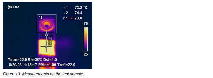
Next thing I do is ask myself: What is the highest emissivity this target could ever have? Well, a blackbody  is 1.0, and nothing ever goes above that. So, what are the consequences of setting 1.0 as the emissivity?  First of all, the camera will no longer include the reflected apparent temperature in the calculation, so  whatever I set it to doesn’t matter. (But I should still avoid actual spot reflections of course!) Assuming  that I measure on a target hotter that the surroundings, the second thing that will happen is that my  temperature measurement will be the absolutely lowest possible from the target. I will be measuring too  low, that is true. BUT I will be able to determine the lowest temperature the target could ever have,  regardless of what the actual emissivity is!  

In this case, using an emissivity of 1.0 on the geometrical shape gives me a “rock-bottom” temperature  reading of 62.5°C, which is higher than any of my guesses above, for the flat surface! Even higher than  my lowest guess of 0.20 for emissivity that gave me 50.2°C. To get the same reading on the flat copper  

surface, I must go down to 0.13 or lower. Personally, I never like to set my camera at emissivities that low  if I have to guess, because it is so sensitive to error that far down.  

Comparing this “rock-bottom” measurement of 62.5°C, which I am 100% sure that the real temperature  will not go under, with the one I got from guessing on the copper, I can easily conclude that my emissivity  guess was definitely wrong.  

How can this be used in practice? Let’s say, for example, that I measure the “rock-bottom” temperature to  be 85°C, and my limit for the highest classification of an anomaly is 80°C. Well, the job is done then, isn’t  it? Any decrease in emissivity will only increase the measured temperature from that point, and it will still  be classified the same!  

If you make a statement about something, your boss or your customer will probably be more impressed  by a measurement you know for sure is not less than the number you are stating, than a very uncertain  value that has a high probability of being very wrong. That is especially true if you will be basing a  decision to shut something down, on that measurement. 

Gambling a little more  

Is it likely that the geometrical shape around the riveted stud will have an emissivity higher that electrical  tape, for example? Probably not, emissivities over 0.95 are rare. So let’s gamble that the emissivity is  0.95, and see what we get. The result is 64.3°C. We get a little closer to the real temperature. (And now  we do have to put in the correct reflected apparent temperature!)  

How about sticking our necks out a bit more and say that it is very unlikely that the emissivity will be  higher than 0.90. That gives us a temperature reading of 66.3°C. That is yet a little closer to the true value  of 73.2°C, without gambling an awful lot. You get the idea. Now decide how much you want to gamble. At  0.85 you will read 68.5°C, and now you are less than 5 K away from the real value. At 0.80, you will  measure 70.9°C. In any case, you will probably be on more solid ground using the geometrical shape  than betting on the low emissivity, flat copper surface. Any gambler likes better odds.  

What is the emissivity of that stud, anyway? Having the correct answer available to us, we can easily  determine that it is 0.76.  

SUMMARY  

If you frequently do thermography and temperature measurements on targets made of metal, and if the  degree of corrosion is often low, and if the surface structure is smooth, you would normally be in a bit of  trouble with emissivity. If that is true for you, it will definitely be worthwhile to learn a little more about the  geometry factor.  

Emissivity due to geometry effects vary more with viewing angle than we would normally expect a flat  surface to do. To make the most use of geometry effects in the field, we need to move around until we  find an angle that shows the highest apparent temperature.  

The lower the emissivity of the material itself is, the more help you will get from geometry. If the surface  emissivity is already high, there is less room for improvement by geometry. For geometry to increase the  emissivity on a high emissivity surface you need a more sophisticated geometrical shape.  

A geometrical shape will always have a higher emissivity than a flat surface, all else being equal.  Measuring on a higher emissivity will always make your guessing of emissivity a gamble with better odds.  So take advantage of those geometrical shapes.  

REFERENCES  

1. Öhman, Claes; “Measurement in Thermography”, FLIR Systems AB, ITC Publ. no.: 1 560 055,  Nov 15, 2001 pp. 72-75.